How to optimize Inverter Efficiency Curves for variable load manufacturing facilities?

Introduction to Manufacturing Power Dynamics

Manufacturing facilities are characterized by highly dynamic and fluctuating electrical loads. Throughout a typical 24-hour cycle, power consumption spikes and sags as production lines start up, CNC machines cycle through cutting routines, air compressors cycle, and facility lighting is switched. Designing an off-grid or back-up power system for such variable environments requires more than just ensuring the system can handle the peak possible load.

To achieve optimal economic performance and minimize utility or fuel costs, systems integrators must analyze the efficiency characteristics of the power electronic inverters. An inverter's efficiency is not static; it changes dramatically depending on the active load. Operating an inverter far outside its optimal efficiency window can result in significant energy waste.

This article delivers a technical breakdown of inverter efficiency curves and explains how to design and optimize multi-inverter systems for fluctuating manufacturing environments.

Question: How can system designers optimize inverter efficiency curves in manufacturing facilities with highly variable loads?

To optimize inverter efficiency curves in variable-load manufacturing facilities, engineers must conduct a thorough electrical load profiling, avoid over-sizing a single massive inverter, implement a modular parallel inverter architecture, and deploy dynamic phase shedding (or master-slave staging). This staging keeps the active inverters operating within their peak efficiency sweet-spots (typically between 50% and 80% of rated capacity) while shifting inactive units into zero-draw sleep modes. Designing with high-performance JYINS industrial inverters ensures maximum efficiency across the entire load spectrum.

The Anatomy of an Inverter Efficiency Curve

To optimize efficiency, we must first understand the mathematical and physical losses that define an inverter's operation. An inverter's efficiency (eta) is calculated as:

eta = ( AC Power Output / DC Power Input )  100%

This ratio is affected by three primary categories of internal power losses, which vary differently across the load range:

• No-Load (Constant) Losses: These are the energy losses required to keep the inverter energized, including control board power, cooling fans, and magnetic core (iron) losses in low-frequency transformers. These losses are completely independent of the load. Under very light loads (e.g., under 10% of rated capacity), constant losses dominate the equation, causing the efficiency curve to plummet to extremely low levels (often below 50%).
• Conduction (I^2  R) Losses: As current (I) flows through the inverter's internal components, such as PCB copper traces, terminal blocks, filter inductors, and the internal channel resistance of the MOSFETs, energy is dissipated as heat. Conduction losses are proportional to the square of the load current. Under high-load conditions (e.g., above 90% capacity), conduction losses increase exponentially, causing the efficiency curve to drop slightly.
• Switching Losses: These are the energy losses that occur in the semiconductor MOSFETs or IGBTs as they transition between the 'ON' and 'OFF' states. Switching losses are proportional to the switching frequency and the voltage. They remain relatively linear across the load range.

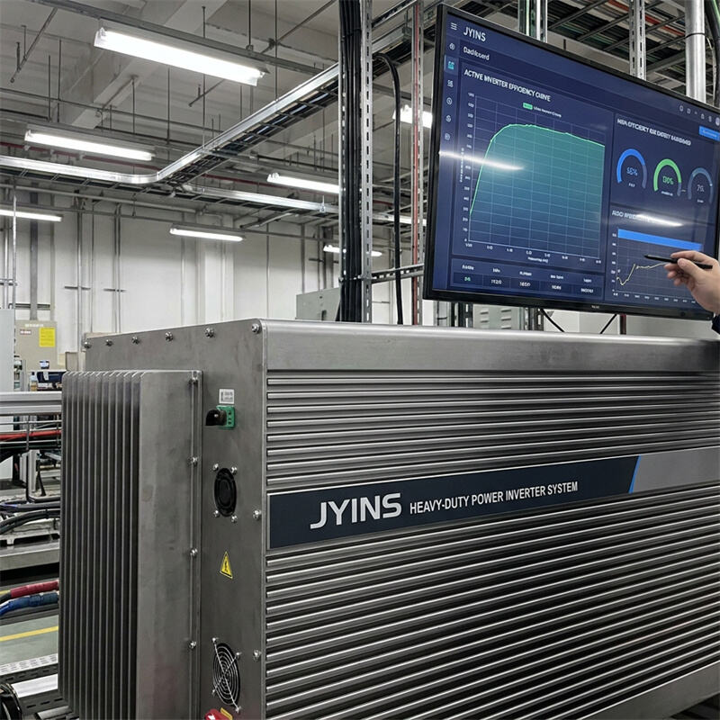
When these losses are plotted on a graph showing Percent Load (X-axis) versus Percent Efficiency (Y-axis), a distinct curve emerges. For a typical high-quality industrial inverter, the peak efficiency (often reaching 93% to 96%) occurs in a sweet-spot between 50% and 80% load. Below 20% load, the efficiency drops off rapidly due to constant losses. Above 90% load, the efficiency dips slightly due to escalating conduction losses.

Sizing Pitfalls in Variable-Load Environments

A common mistake among systems integrators is sizing a single, massive inverter based on the absolute peak startup demand of the facility.

For example, if a workshop has a peak startup spike of 30 kW when a massive dust extractor is turned on, but spends 90% of its working day drawing a continuous background load of only 3 kW, the designer might install a single 40 kW inverter.

While this 40 kW inverter easily handles the 30 kW spike, for the vast majority of the day it is operating at only:

( 3 kW / 40 kW )  100% = 7.5% load.

At 7.5% load, the inverter's efficiency is extremely low—likely around 65% due to its high internal idle consumption (which might be 200W of constant draw). This means the system is wasting massive amounts of energy throughout the day, requiring larger solar arrays and accelerating battery wear. This is known as 'over-sizing inefficiency'.

Engineering Strategies for Efficiency Optimization

To solve this, modern industrial designers employ several advanced system-level strategies:

• 1. High-Resolution Load Profiling

Before selecting hardware, install a power quality meter to log the facility's active load (kW) and apparent load (kVA) at 1-minute intervals over a standard week. Identify the base idle load, the average operating load, and the duration and frequency of peak startup surges. This data maps the target operating zone for the inverter system.

• 2. Modular Parallel Inverter Stacking

Instead of a single 40 kW inverter, a modular system using four 10 kW JYINS parallel-capable inverters is the professional choice. When the facility is running at its average 8 kW daytime load, the system can distribute the load. More importantly, it can dynamically disable unnecessary units.

• 3. Dynamic Phase Shedding (Master-Slave Staging)

In a smart modular system connected via high-speed parallel communication, the system controller monitors active load demand in real-time.

• Under 8 kW of load, only a single 10 kW 'master' inverter remains active. This master unit is loaded at 80% capacity, placing it squarely in its peak 94% efficiency sweet-spot.
• The remaining three 10 kW 'slave' inverters are placed in a zero-draw sleep mode, eliminating their constant no-load losses.
• When the dust extractor starts and the load spikes to 28 kW, the controller instantly wakes up the three sleeping inverters (within milliseconds) to support the load. Once the surge passes and the load drops back, the slaves are placed back to sleep. This dynamic staging maximizes system efficiency across the entire 24-hour cycle.
• 4. Split-Bus Distribution for Scheduled Loads

If certain high-power machines are only operated at specific times (e.g., high-temperature curing ovens used once a week), wire these machines to a dedicated, isolatable AC sub-distribution panel. This sub-panel can be powered by a dedicated inverter bank that is physically shut down via contactors when not in use, ensuring that the main inverter bank is never over-sized for the daily baseline load.

Conclusion

Optimizing inverter efficiency curves in variable-load manufacturing facilities is a critical step in reducing operating costs and enhancing power system reliability. By understanding the physical drivers of inverter loss—no-load losses under light loads and conduction losses under heavy loads—designers can avoid the trap of single-unit over-sizing. Implementing a modular parallel inverter architecture using JYINS industrial hardware, and configuring master-slave dynamic phase staging, ensures that the system always operates within its peak efficiency sweet-spot. This active energy management protects capital investments, optimizes battery utilization, and delivers substantial long-term financial savings.